Machine learning in Julia: Titanic
Published:
Introduction
In this article I will describe my first experiment using Julia for machine learning. I will use the Titanic dataset from Kaggle as the example.
Which IDE
I experimented with 3 different environments to do machine learning in Julia
- VS code
- Pluto.jl
- JupyterLab
VS Code works fine with Julia, but for machine learning it makes sense if you can experiment a lot with settings, so a solutions where you can run updates on individual lines of codes is preferred. I then tried Pluto.jl: it works great and the feedback what’s happening in the background is great. The only downside is that by default you only can have 1 statement per cell. JupyterLab does allow multiple statements per cell, but that requires installing Python even though I want to program in Julia ! Also the feedback what’s happening is not as detailed/nice as in Pluto.jl. In the end I settled on using VS Code with .ipynb (=Jupyter notebook files). Basically you get the benefits of Jupyter without installing Jupiter.
Load data
Let’s start by reading the data from CSV files and load them in DataFrames
using CSV, DataFrames, CategoricalArrays, Statistics, MLJ, MLJDecisionTreeInterface, TableTransforms,Flux, CUDA, Plots

train = "C:\Git\juliacode\Data\titanic-data\train.csv"
test = "C:\Git\juliacode\Data\\titanic-data\test.csv"

df_train = DataFrame(CSV.File(train))
df_test = DataFrame(CSV.File(test))

describe(df_train)
12×7 DataFrame
Row │ variable mean min median max ⋯
│ Symbol Union… Any Union… Any ⋯
─────┼──────────────────────────────────────────────────────────────────────────
1 │ PassengerId 446.0 1 446.0 891 ⋯
2 │ Survived 0.383838 0 0.0 1
3 │ Pclass 2.30864 1 3.0 3
4 │ Name Abbing, Mr. Anthony van Melkebeke, Mr.
5 │ Sex female male ⋯
6 │ Age 29.6991 0.42 28.0 80.0
7 │ SibSp 0.523008 0 0.0 8
8 │ Parch 0.381594 0 0.0 6
9 │ Ticket 110152 WE/P 5735 ⋯
10 │ Fare 32.2042 0.0 14.4542 512.329
11 │ Cabin A10 T
12 │ Embarked C S
3 columns omittedLet’s check the types of the data in each of the columns
schema(df_train)┌─────────────┬────────────────────────────┬──────────────────────────┐
│ names │ scitypes │ types │
├─────────────┼────────────────────────────┼──────────────────────────┤
│ PassengerId │ Count │ Int64 │
│ Survived │ Count │ Int64 │
│ Pclass │ Count │ Int64 │
│ Name │ Textual │ String │
│ Sex │ Textual │ String7 │
│ Age │ Union{Missing, Continuous} │ Union{Missing, Float64} │
│ SibSp │ Count │ Int64 │
│ Parch │ Count │ Int64 │
│ Ticket │ Textual │ String31 │
│ Fare │ Continuous │ Float64 │
│ Cabin │ Union{Missing, Textual} │ Union{Missing, String15} │
│ Embarked │ Union{Missing, Textual} │ Union{Missing, String1} │
└─────────────┴────────────────────────────┴──────────────────────────┘schema(df_test)┌─────────────┬────────────────────────────┬──────────────────────────┐
│ names │ scitypes │ types │
├─────────────┼────────────────────────────┼──────────────────────────┤
│ PassengerId │ Count │ Int64 │
│ Pclass │ Count │ Int64 │
│ Name │ Textual │ String │
│ Sex │ Textual │ String7 │
│ Age │ Union{Missing, Continuous} │ Union{Missing, Float64} │
│ SibSp │ Count │ Int64 │
│ Parch │ Count │ Int64 │
│ Ticket │ Textual │ String31 │
│ Fare │ Union{Missing, Continuous} │ Union{Missing, Float64} │
│ Cabin │ Union{Missing, Textual} │ Union{Missing, String15} │
│ Embarked │ Textual │ String1 │
└─────────────┴────────────────────────────┴──────────────────────────┘I created a function to prepare the data and select the features to be used in the machine learning step. I selected the columns which I expect to be most relevant and recode them such that they are all numeric. Finally I apply ZScore to scale the features.
function preprocess(df)
    #select columns
    # df2 = df[:, [:PassengerId, :Pclass, :Sex, :SibSp, :Parch]]

    df2 = select(df,
        Not(
            ["PassengerId", "Name", "Ticket", "Cabin"]
        )
    )

    df2.Embarked = replace(
        df2.Embarked, "S" => 1, "C" => 2, "Q" => 3
    )
    recode!(df2.Embarked , missing => 0)
    df2.Embarked= convert.(Int64,df2.Embarked)
    df2.Embarked = disallowmissing(df2.Embarked)

    #remove missings from Age
    age = df.Age
    recode!(age, missing => mean(skipmissing(age)))
    df2[:, :Age] = age
    df2.Age = disallowmissing(df2.Age)

    #remove missings from Fare
    fare = df.Fare
    recode!(fare, missing => mean(skipmissing(fare)))
    df2[:, :Fare] = fare
    df2.Fare = disallowmissing(df2.Fare)

    #recode Sex from String to boolean
    df2.Sex = ifelse.(df2.Sex .== "male", 0, 1)
    # f1 = Coerce(:Pclass => Continuous, :Sex => Continuous)
    # df2 = df2 |> f1
    f2 = ZScore( :Fare,:Age )
    df2 = df2 |> f2

    passengerId = df[:,"PassengerId"]
    passengerId, df2
end
preprocess (generic function with 1 method)Then I process the training set and the test set..
passengerIdTrain, df_train2 = preprocess(df_train);
passengerIdTest, df_test2 = preprocess(df_test);
df_train2[:, :Survived] = df_train.Survived;
coerce!(df_train2, :Survived => Multiclass);
schema(df_train2)
y, X = unpack(df_train2, ==(:Survived); rng=123)
(CategoricalArrays.CategoricalValue{Int64, UInt32}[1, 0, 0, 0, 1, 0, 0, 1, 1, 1 … 1, 0, 0, 0, 0, 1
, 0, 0, 1, 0], 891×7 DataFrame
Row │ Pclass Sex Age SibSp Parch Fare Embarked
│ Int64 Int64 Float64 Int64 Int64 Float64 Int64
─────┼───────────────────────────────────────────────────────────────
1 │ 3 1 0.100052 0 0 -0.47332 1
2 │ 3 0 -2.13037 4 1 -0.0619641 3
3 │ 3 0 0.0 0 0 -0.489167 1
4 │ 2 0 0.330786 1 0 -0.12485 1
5 │ 1 1 1.86901 1 0 0.926933 2
6 │ 3 0 0.0615968 0 0 -0.486064 1
7 │ 3 0 0.176964 0 0 -0.479776 1
8 │ 3 0 0.176964 0 0 -0.486064 1
⋮ │ ⋮ ⋮ ⋮ ⋮ ⋮ ⋮ ⋮
885 │ 3 0 -0.476781 0 0 -0.502582 2
886 │ 3 0 -0.130681 0 0 -0.489167 1
887 │ 1 1 -1.13053 0 1 3.60477 1
888 │ 2 0 -0.515237 0 0 -0.386454 1
889 │ 3 0 -0.822881 0 0 -0.648058 1
890 │ 3 0 1.0999 0 0 -0.48858 1
891 │ 3 0 0.0 0 0 -0.492101 3
876 rows omitted)schema(df_train2)┌──────────┬───────────────┬─────────────────────────────────┐
│ names │ scitypes │ types │
├──────────┼───────────────┼─────────────────────────────────┤
│ Survived │ Multiclass{2} │ CategoricalValue{Int64, UInt32} │
│ Pclass │ Count │ Int64 │
│ Sex │ Count │ Int64 │
│ Age │ Continuous │ Float64 │
│ SibSp │ Count │ Int64 │
│ Parch │ Count │ Int64 │
│ Fare │ Continuous │ Float64 │
│ Embarked │ Count │ Int64 │
└──────────┴───────────────┴─────────────────────────────────┘For this experiment I will use a Random Forest classifier. Using ‘evaluate’ I can check how well it does on the training set. Better results might be achievable when using different classifiers.
RandomForest = @load RandomForestClassifier pkg = DecisionTree
randomForest = RandomForest()
evaluate(randomForest, X, y,
    resampling=CV(shuffle=true),
    measures=[log_loss, MLJ.accuracy],
    verbosity=0)
import MLJDecisionTreeInterface ✔
PerformanceEvaluation object with these fields:
measure, operation, measurement, per_fold,
per_observation, fitted_params_per_fold,
report_per_fold, train_test_rows
Extract:
┌────────────────────────────────┬──────────────┬─────────────┬─────────┬───────
│ measure │ operation │ measurement │ 1.96*SE │ per_ ⋯
├────────────────────────────────┼──────────────┼─────────────┼─────────┼───────
│ LogLoss( │ predict │ 0.661 │ 0.283 │ [0.3 ⋯
│ tol = 2.220446049250313e-16) │ │ │ │ ⋯
│ Accuracy() │ predict_mode │ 0.82 │ N/A │ [0.8 ⋯
└────────────────────────────────┴──────────────┴─────────────┴─────────┴───────
1 column omittedFinally I create a machine using the Random Forest classifier and train it on the test set. Then I can use that machine to predict the survivors in the test set. The score on Kaggle was 0.77272
mach = machine(randomForest, X, y)
MLJ.fit!(mach);
yhat = predict_mode(mach, df_test2)
dfOut = DataFrame();

dfOut[:, :PassengerId] = passengerIdTest;
dfOut[:, :Survived] = yhat;
dfOut
output = "C:\Git\juliacode\Data\titanic-data\submissionRandomForest.csv"
CSV.write(output, dfOut)"C:\Git\juliacode\Data\titanic-data\submissionRandomForest.csv"Neural network
Neural networks are not very well suited for small datasets like the Titanic dataset, but let’s check how it compares again the RandomForest classifier
model = Chain(
    Dense(size(X,2) => size(X,2)),
    Dense(size(X,2) => size(X,2)),
    Dense(size(X,2) => 2),
    softmax
    ) |> gpu
Chain(
Dense(7 => 7), # 56 parameters
Dense(7 => 7), # 56 parameters
Dense(7 => 2), # 16 parameters
NNlib.softmax,
) # Total: 6 arrays, 128 parameters, 856 bytes.target = Flux.onehotbatch(y, [0,1])2×891 OneHotMatrix(::Vector{UInt32}) with eltype Bool:
⋅ 1 1 1 ⋅ 1 1 ⋅ ⋅ ⋅ 1 1 1 … 1 1 ⋅ 1 1 1 1 ⋅ 1 1 ⋅ 1
1 ⋅ ⋅ ⋅ 1 ⋅ ⋅ 1 1 1 ⋅ ⋅ ⋅ ⋅ ⋅ 1 ⋅ ⋅ ⋅ ⋅ 1 ⋅ ⋅ 1 ⋅loader = Flux.DataLoader((collect(Matrix(X)'), target) |> gpu, batchsize=32, shuffle=true)28-element DataLoader(::Tuple{CUDA.CuArray{Float32, 2, CUDA.Mem.DeviceBuffer}, OneHotArrays.OneHotMa
trix{UInt32, CUDA.CuArray{UInt32, 1, CUDA.Mem.DeviceBuffer}}}, shuffle=true, batchsize=32)
with first element:
(7×32 CUDA.CuArray{Float32, 2, CUDA.Mem.DeviceBuffer}, 2×32 OneHotMatrix(::CUDA.CuArray{UInt32, 1,
CUDA.Mem.DeviceBuffer}) with eltype Bool,)optim = Flux.setup(Flux.Adam(), model)(layers = ((weight = Leaf(Adam{Float64}(0.001, (0.9, 0.999), 1.0e-8), (Float32[0.0 0.0 … 0.0 0.0; 0.
0 0.0 … 0.0 0.0; … ; 0.0 0.0 … 0.0 0.0; 0.0 0.0 … 0.0 0.0], Float32[0.0 0.0 … 0.0 0.0; 0.0 0.0 … 0.0
0.0; … ; 0.0 0.0 … 0.0 0.0; 0.0 0.0 … 0.0 0.0], (0.9, 0.999))), bias = Leaf(Adam{Float64}(0.001, (0
.9, 0.999), 1.0e-8), (Float32[0.0, 0.0, 0.0, 0.0, 0.0, 0.0, 0.0], Float32[0.0, 0.0, 0.0, 0.0, 0.0, 0
.0, 0.0], (0.9, 0.999))), σ = ()), (weight = Leaf(Adam{Float64}(0.001, (0.9, 0.999), 1.0e-8), (Float
32[0.0 0.0 … 0.0 0.0; 0.0 0.0 … 0.0 0.0; … ; 0.0 0.0 … 0.0 0.0; 0.0 0.0 … 0.0 0.0], Float32[0.0 0.0
… 0.0 0.0; 0.0 0.0 … 0.0 0.0; … ; 0.0 0.0 … 0.0 0.0; 0.0 0.0 … 0.0 0.0], (0.9, 0.999))), bias = Leaf
(Adam{Float64}(0.001, (0.9, 0.999), 1.0e-8), (Float32[0.0, 0.0, 0.0, 0.0, 0.0, 0.0, 0.0], Float32[0.
0, 0.0, 0.0, 0.0, 0.0, 0.0, 0.0], (0.9, 0.999))), σ = ()), (weight = Leaf(Adam{Float64}(0.001, (0.9,
0.999), 1.0e-8), (Float32[0.0 0.0 … 0.0 0.0; 0.0 0.0 … 0.0 0.0], Float32[0.0 0.0 … 0.0 0.0; 0.0 0.0
… 0.0 0.0], (0.9, 0.999))), bias = Leaf(Adam{Float64}(0.001, (0.9, 0.999), 1.0e-8), (Float32[0.0, 0
.0], Float32[0.0, 0.0], (0.9, 0.999))), σ = ()), ()),)losses = []
for epoch in 1:100
for (x, y) in loader
loss, grads = Flux.withgradient(model) do m
# Evaluate model and loss inside gradient context:
y_hat = m(x)
Flux.crossentropy(y_hat, y)
end
Flux.update!(optim, model, grads[1])
push!(losses, loss) # logging, outside gradient context
end
end
plot(losses)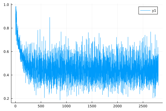
target_hat = model(collect(Matrix(X)') |> gpu) |> cpu
(Flux.onecold(target_hat) .- 1)'
1×891 adjoint(::Vector{Int64}) with eltype Int64:
1 0 0 0 1 0 0 0 1 1 0 1 0 … 0 0 1 0 0 0 0 1 0 0 0 0function accuracy(y_hat, y_raw)
y_hat_raw = Flux.onecold(y_hat) .- 1
count(y_hat_raw .== y_raw) / length(y_raw)
end
y_hat2 = Flux.onecold(target_hat) .- 1
accuracy(target_hat,y)0.8047138047138047y_test = Flux.onecold( model(collect(Matrix(df_test2)') |> gpu) |> cpu ) .- 1418-element Vector{Int64}:
0
0
0
0
1
0
1
0
1
0
⋮
1
1
1
1
0
1
0
0
0dfOut[:, :PassengerId] = passengerIdTest;
dfOut[:, :Survived] = y_test;
output = "C:\Git\juliacode\Data\titanic-data\submissionNeuralNetwork.csv"
CSV.write(output, dfOut)"C:\Git\juliacode\Data\titanic-data\submissionNeuralNetwork.csv"Conclusion
Machine learning in Julia is as easy as in Python. The RandomForest classifier works quite well on the Titanic dataset. The neural network classifier I designed doesn’t give better results then the RandomForest classifier